A step-by-step explanation of the U-Net architecture, the problem pressures that shaped it, and why it remains a serious baseline for many dense prediction tasks.
A reproducible image-to-image benchmark pipeline built on the BSCCM dataset. The project uses 23 label-free microscopy views to predict 6 fluorescence channels, with an emphasis on controlled data handling, explicit run configuration, and stable evaluation before broader model comparisons.
Dense prediction asks a model to do something harder than image classification. It must say what is present, but it must also say where exactly it is present. That sounds small on paper. In practice, it creates one of the core tensions in vision.
A model needs broad context to recognize structures correctly. It also needs fine detail to place boundaries in the right pixels. Those two goals pull in opposite directions. If the model looks only at tiny local patches, it may miss the larger structure. If it compresses too aggressively to gain context, it may lose the very detail needed for precise localization.
U-Net became important because it responds directly to that tension.1 Its shape is not arbitrary. The contracting path builds context. The expanding path recovers spatial precision. The skip connections help the model combine the two. If you understand that, the architecture stops looking like a diagram to memorize and starts looking like a solution to a real problem.
What dense prediction actually needs
In image classification, the final answer can be one label for the whole image. A cat is a cat whether it appears in the top-left or bottom-right. Dense prediction is different. The output must stay aligned with the input. Every location matters.
That means the model must preserve spatial meaning throughout the computation. It cannot simply collapse the image into a single decision and call the job done. It has to return a map. In segmentation, that map may be a class prediction for each pixel. In dense regression, it may be a continuous value at each location. Either way, the prediction remains spatial.
This is why dense prediction is not solved by just making a classifier deeper. The model must understand structure at multiple scales. It has to see local edges, medium-sized shapes, and larger spatial context. It also has to keep those levels coordinated well enough that the final map is sharp rather than vague.
That problem setting is the right starting point for U-Net. Before talking about convolutions, pooling, or skip connections, it helps to hold onto one anchor idea:
Dense prediction needs broad context and precise localization at the same time.
Everything else in the architecture follows from that.
The central idea of U-Net
The original U-Net paper describes the architecture as a contracting path on the left and an expansive path on the right.1 That is the whole design in one sentence.
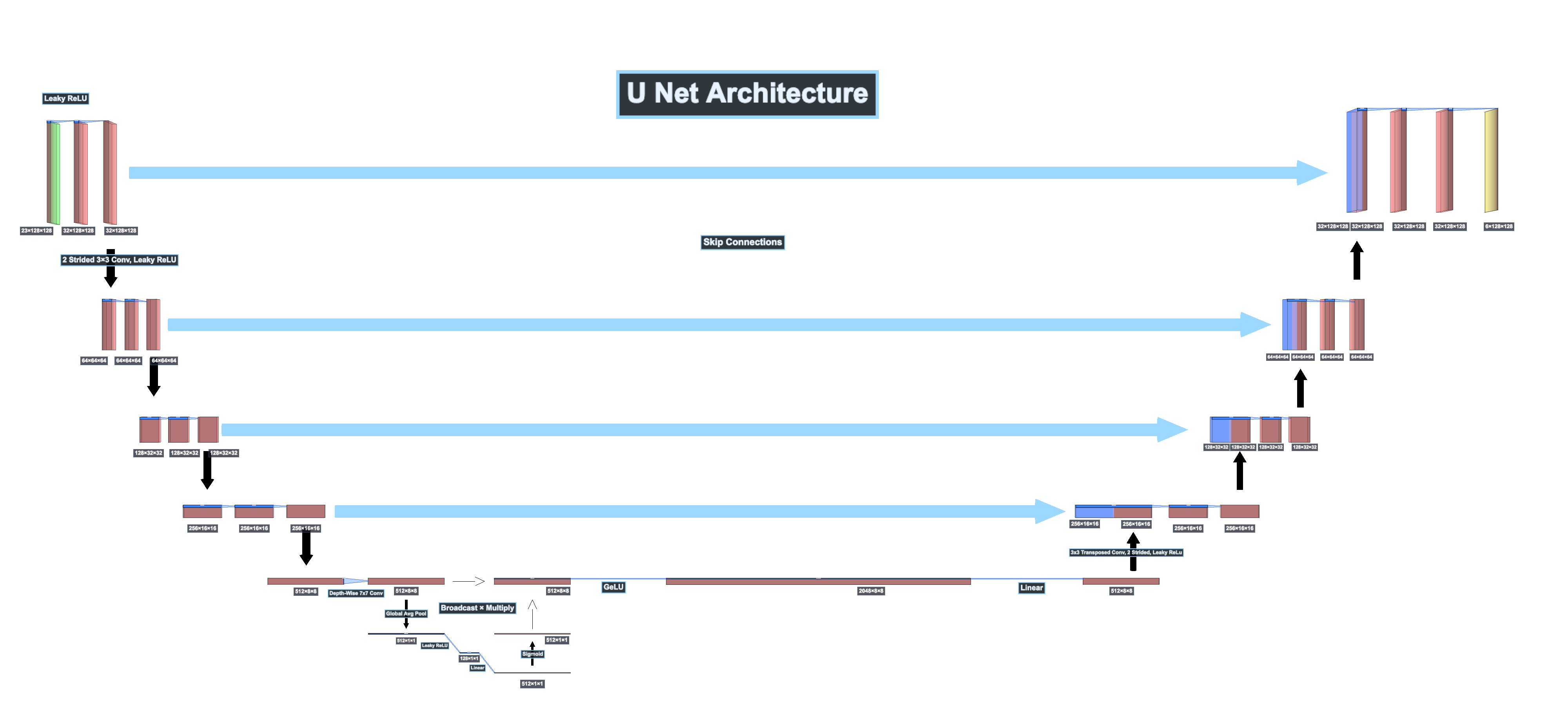
The left side gradually reduces spatial resolution. As it goes deeper, the representation becomes smaller in width and height but richer in channels. This helps the network build broader context. The model can reason over larger neighborhoods and represent more abstract structure.
The right side gradually raises the spatial resolution again. This is not just an undo button. It is a reconstruction path. It tries to turn the compressed, high-context representation into a dense output that is spatially precise.
If the architecture stopped there, it would already be a reasonable encoder-decoder. But U-Net adds the part that made it especially effective: skip connections between matching resolutions on the left and right sides.1 Those links give the decoder access to higher-resolution features that would otherwise be lost.
So the “U” is not only a shape. It is a statement about the computation. The model first compresses to understand. Then it expands to localize. And during that expansion, it reaches back to recover detail.
U-Net architecture view showing how the contracting path builds context, the bottleneck
compresses representation, and the expanding path recovers localization with skip-connected
features.
The contracting path
The contracting path is where U-Net gathers context. In the original paper, each stage applies two 3×3 unpadded convolutions, each followed by ReLU, and then a 2×2 max-pooling operation with stride 2 for downsampling.1 At every downsampling step, the number of feature channels doubles.1
It helps to slow that down.
The first convolutions near the input operate at full or near-full resolution. They begin by turning raw pixel patterns into simple learned features. Those may respond to edges, intensity transitions, texture fragments, or other local structures. The next convolution can combine those signals into slightly richer local patterns.
Then pooling reduces the spatial size of the feature map. This matters for two reasons. First, it increases the effective spatial reach of later layers. A deeper layer can now reason over a larger region of the original image. Second, smaller feature maps make it affordable to increase channel count. The network can store richer feature descriptions even while the map becomes spatially smaller.
This is the main trade in the encoder:
the model gives up exact spatial precision in exchange for broader contextual understanding.
That trade is not a flaw. It is necessary. A segmentation model still needs to know whether a local patch belongs to a membrane, nucleus, gland, organ, or background region in a larger structure. Local evidence alone is often ambiguous.
But the cost is real. The deeper the model goes, the less natural access it has to the exact high-resolution boundaries present at the input. That cost is what the rest of U-Net is designed to manage.
The bottleneck
The bottleneck is the lowest-resolution part of the network. It is where the representation is most compressed and most semantic.
That does not mean it contains a magical “essence” of the image. It means something simpler and more useful. At this point, the network has gathered strong contextual information, but it has the weakest direct access to fine-grained spatial detail.
This matters because dense prediction cannot be solved from semantics alone. A model may know that a certain region likely contains a cell, tissue boundary, or organ. That still does not tell it where the exact boundary should be drawn pixel by pixel.
So the bottleneck is powerful and limited at the same time. It is powerful because it sees a lot of context. It is limited because localization has already been compressed away. This is why the decoder is necessary. The model cannot stop at the bottleneck and still expect precise segmentation.
The expanding path
In the original U-Net, every decoder stage upsamples the feature map, applies a 2×2 up-convolution that halves the number of channels, concatenates the result with a correspondingly cropped encoder feature map, and then applies two more 3×3 convolutions with ReLU.1
The key point here is easy to miss:
upsampling alone does not restore information that was lost.
Making a feature map larger does not magically recover sharp object boundaries. It only increases the spatial size of the representation. The real work of the decoder is not simple resizing. The real work is reconstruction and refinement.
At each stage, the decoder takes a coarse, context-rich representation and moves it toward a finer spatial map. The upsampled decoder features carry the model’s current understanding of what structures are likely present. But they are still coarse. They need help to become precise.
That help comes from the skip connections.
Skip connections
Skip connections are one of the central reasons U-Net works well. They copy feature maps from the encoder to the decoder at matching resolutions, where those features are concatenated with the upsampled decoder features.1
This is not just a convenient shortcut. It solves the exact problem created by downsampling.
During the contracting path, the model learns useful high-resolution features before pooling reduces spatial detail. Those features contain information that may later be very hard to reconstruct from the bottleneck alone. When the decoder returns to that scale, the skip connection brings those higher-resolution features back into play.
That gives the decoder two kinds of information at once.
The upsampled decoder features provide coarse semantic context. They help answer questions like: what broad structure is likely present here?
The encoder features provide finer spatial detail. They help answer questions like: where should the edge actually go?
U-Net does not choose between those two sources. It concatenates them and lets the following convolutions learn how to fuse them.1 That last part matters. Concatenation is not the final answer. The fusion happens in the layers that follow.
This is why skip connections should not be explained as “passing information forward” and left at that. They exist because dense prediction needs detail that pooling would otherwise discard.
Shape bookkeeping is part of the architecture
One of the most educational details in the original U-Net is that it uses unpadded 3×3 convolutions.1 That means every convolution shrinks the spatial dimensions of the feature map. This choice has consequences.
First, the output is smaller than the input.1 The paper explicitly notes that due to unpadded convolutions, the output image is smaller than the input by a constant border width.1
Second, the skip-connected feature maps from the encoder cannot always be concatenated directly with the decoder maps. Their shapes do not automatically line up. The original model handles this by cropping the encoder features before concatenation.1
That cropping is not a random implementation detail. It is the geometric consequence of a design choice. This is a good reminder that architecture diagrams are not just abstract graphs. They are shape-transforming systems. Padding, pooling, and upsampling decisions affect how information can actually be aligned and fused.
The original paper also pairs this design with an overlap-tile strategy and mirrored borders so the network can segment large images seamlessly.1 That is another example of architecture and deployment details being tightly connected.
The final output layer
At the end of the network, U-Net uses a 1×1 convolution to map each feature vector at a spatial location to the desired number of output classes.1 This is the final translation from internal representation to task prediction.
It helps to say this plainly. By the time the decoder reaches the final resolution, each location in the feature map holds a learned vector of features. That vector is rich, but it is still internal. The last layer turns that vector into something task-specific.
For segmentation, that usually means one score per class at each location. For a binary task, it may be foreground versus background. For a multi-class task, it may be a logit vector over all classes. For dense regression, it may be one or more continuous outputs per location.
The 1×1 convolution is useful because it mixes channels at the same location without mixing neighboring locations spatially. By that point, the spatial reasoning has already happened. The final layer performs the output projection.
Training choices were part of the original success
It is tempting to talk about U-Net as if the architecture alone explains everything. The original paper makes clear that this would be incomplete.1
One major ingredient was data augmentation. The authors state that data augmentation is essential when only a few training samples are available, and they describe random elastic deformations as a key concept for training a segmentation network with very few annotated images.1 That matters a lot in biomedical imaging, where dense labels are expensive.
Another important ingredient was the weighted loss map used to emphasize the narrow borders between touching cells.1 The paper explicitly introduces large weights for separating background labels between touching objects so the model learns those difficult borders better.1 This is not cosmetic. In many cell segmentation tasks, separating adjacent instances is one of the hardest parts of the problem.
The paper also ties its architecture to a practical inference strategy for large images.1 That is easy to ignore in simplified retellings, but it is part of why the model was useful in practice.
So a fair reading of U-Net is this: the architecture was strong, but the training setup and inference design were also tightly matched to the problem.
A forward pass from start to finish
One way to make U-Net feel intuitive is to follow one image through the whole network.
The input enters at full resolution. Early convolutions detect local patterns and simple structures.
The contracting path then repeats a rhythm: convolve, convolve, downsample. At each new level, the model sees a broader effective neighborhood and carries richer feature channels, but the map becomes spatially coarser.
By the bottleneck, the representation is compact and strongly contextual. The model has a better sense of larger structure, but fine localization is no longer easy.
The decoder begins to raise the spatial resolution again. At each stage, the model upsamples the current representation and combines it with encoder features from the matching scale. Those encoder features reintroduce spatial detail that was present before pooling.
The post-concatenation convolutions then fuse the context-rich decoder signal with the detail-rich encoder signal. This process repeats scale by scale until the representation is again close to the desired output resolution.
Finally, the 1×1 output layer maps each location’s refined feature vector into the prediction space.
That is the whole motion of U-Net: compress for context, expand for localization, and repeatedly fuse the two.
Why U-Net became such a strong baseline
U-Net became influential because its inductive bias fit the problem well.1 It was not just early. It was well-shaped for biomedical dense prediction.
The original paper made a very concrete claim. The architecture uses a contracting path to capture context and a symmetric expanding path to enable precise localization, and with strong augmentation it can be trained end-to-end from very few images.1 The results were also concrete. On the EM segmentation challenge, the paper reported a new best warping error, and on ISBI cell tracking segmentation tasks it reported strong IoU gains over prior methods.1
That combination mattered. The model was not only conceptually elegant. It also worked under realistic biomedical constraints: limited annotated data, strong need for localization, and frequent need to separate touching structures.
What is especially interesting is that the broader field has continued to validate U-Net as a serious baseline rather than merely a historical artifact. nnU-Net showed that a carefully configured U-Net-based pipeline, with automated handling of preprocessing, architecture, training, and post-processing, could surpass most existing approaches on 23 public biomedical segmentation datasets without manual intervention.2 That is a remarkable result because it shifts attention away from novelty alone and toward careful system design.
The later nnU-Net Revisited paper pushes this point even harder. It argues that many claims of superiority over U-Net fail under more rigorous validation, and it concludes that the recipe for state-of-the-art performance still relies on CNN-based U-Net models, the nnU-Net framework, and scaling to modern hardware.3
So when people say “U-Net is still a good baseline,” the mature version of that statement is stronger than it sounds. It means that a properly implemented U-Net-family system still deserves to be the reference point many new methods must beat.
Where plain U-Net starts to struggle
A good baseline is not a universal solution. U-Net has real limits.
One limitation comes from long-range dependency modeling. Convolutions are local operations, and while stacking layers and pooling increases effective context, the architecture is still built around local receptive patterns. Later work such as TransUNet explicitly frames this as a weakness of plain U-Net and introduces transformer components to model broader global context more directly.4
Another limitation appears in crowded or instance-heavy settings. Plain semantic segmentation is not always enough when touching objects must be separated cleanly as distinct instances. The original paper already recognized part of this difficulty by weighting border regions more heavily during training.1 That tells us something important: the problem was not fully solved by the basic architecture alone.
A third limitation is that U-Net is not the most representative baseline for every dense-prediction domain. In biomedical imaging, it is often the natural reference point. In other areas of computer vision, different architectural traditions may be more central.
So the honest position is not “U-Net solves dense prediction.” The honest position is:
U-Net solves an important and influential slice of dense prediction very well, and it remains worth understanding because later improvements often modify its weaknesses rather than discard its core logic.
How later variants build on the same logic
Many later architectures do not reject U-Net. They keep its core shape and try to fix specific weaknesses.
UNet++ argues that the encoder and decoder feature maps can be too far apart semantically, so it redesigns the skip pathways using nested dense connections and reports average IoU gains over both U-Net and wide U-Net across several medical segmentation tasks.5 That is a refinement of the skip-fusion story, not a rejection of it.
Attention U-Net adds attention gates so the network can focus more selectively on relevant regions and suppress irrelevant ones, while keeping the U-Net backbone.6 Again, the core encoder-decoder-plus-skip idea remains.
TransUNet makes a different move. It argues that pure transformer encoding loses low-level details if used naively, and then combines transformer-based global context with U-Net-style decoding and high-resolution feature fusion for precise localization.4 That is especially revealing. Even some of the architectures positioned as alternatives still rely on the core insight that made U-Net strong in the first place: dense prediction needs context and localization to be fused, not traded off absolutely.
This is one reason U-Net is such a good architecture to study. It is not just a historical milestone. It is also the backbone of a whole family of later ideas.
Final takeaway
U-Net is worth understanding because it is one of the clearest examples of an architecture whose shape matches the structure of the problem it is solving.
Dense prediction needs broad context. That is why U-Net contracts.
Dense prediction also needs precise localization. That is why U-Net expands.
Dense prediction suffers when detail is lost during compression. That is why U-Net uses skip connections.
And dense prediction becomes much more believable when the architecture, training setup, and evaluation protocol all fit the task rather than chasing novelty for its own sake. That broader lesson is one reason U-Net still matters today.23
If I had to summarize the architecture in one sentence, it would be this:
U-Net became influential because it turns the central tension of dense prediction into a concrete design: compress to understand, recover to localize, and fuse context with detail at every scale.