Why deep networks need nonlinearity

Deep networks are often described as powerful function approximators, but the source of that power is easy to misunderstand. A standard neural network layer applies a linear transformation plus a bias term. Even the most common activation, ReLU, is linear on one side and zero on the other. So the natural question is not just whether nonlinearity matters, but why it matters so much. If the pieces look so simple, where does the expressive power actually come from?

The answer is structural. If every layer in a deep network is linear, the entire network collapses into one global linear rule, no matter how many layers it has. Nonlinearity prevents that collapse. In ReLU networks, this happens through input-dependent gating. Different inputs activate different subsets of units, which partitions the input space into regions. Inside each region the network behaves like a simple linear model, but across regions it can switch to different local rules. That is the step that allows deep networks to represent functions and decision boundaries that one global linear rule cannot.

A network is a composition of functions

At the most basic level, a neural network is a function built by composing simpler functions. A single layer takes an input vector $x$, multiplies it by a weight matrix $W$, adds a bias vector $b$, and produces

$$z = Wx + b$$

If we stack layers, the output of one becomes the input of the next. With two layers and no activation function, the computation looks like this:

$$h_1 = W_1x + b_1$$ $$h_2 = W_2h_1 + b_2$$

This is the basic object we need to think about. A deep network is not magic. It is repeated function composition. The real question is what kinds of functions remain possible after repeated composition, and what kinds do not.

If every layer is linear, depth does not buy a richer function

Now substitute the first equation into the second:

$$h_2 = W_2(W_1x + b_1) + b_2$$ $$h_2 = (W_2W_1)x + (W_2b_1 + b_2)$$

This still has exactly the same form as a single layer: one linear transformation plus one bias term. The same argument extends to any number of layers. If every stage in the network is linear, then the full network can always be rewritten as

$$f(x) = Wx + b$$

for some effective matrix $W$ and bias $b$.

This is the first central fact behind the whole topic. Stacking linear layers does not create a new kind of model. It only creates a more complicated way of writing the same global rule. The depth may look impressive in the architecture diagram, but from the point of view of the function class, nothing fundamentally new has happened.

This is why nonlinearity is not an optional detail. Without it, a deep network is still just one global linear model.

What one global linear rule means

It helps to slow down here and ask what such a model can actually represent.

In regression, a linear model predicts a target value using one fixed weighted combination of the input features:

$$\hat{y} = w^\top x + b$$

That means the same basic relationship holds everywhere in input space. If one feature increases by a certain amount, its effect on the prediction is governed by the same coefficient no matter what other context the input lies in. The model has one global slope pattern.

In classification, a linear model also computes a score of the same form:

$$f(x) = w^\top x + b$$

The decision boundary is the set of points where that score is zero:

$$w^\top x + b = 0$$

In two dimensions this boundary is a line. In three dimensions it is a plane. In higher dimensions it is a hyperplane. So for classification, one global linear rule means one flat cut through the input space.

That is the geometric meaning of linearity here. The model does not bend, switch, or adapt its rule from one region to another. It applies one rule everywhere.

Why that is too weak for many real problems

This limitation shows up in both regression and classification.

For regression, a single global linear rule cannot naturally capture curvature, saturation, thresholds, or strong interactions between variables. If the true relationship looks like $y = x^2$, then no single line can represent it over a broad range. If the effect of one variable changes depending on another, a pure linear model still tries to explain everything through one fixed additive rule. It has no built-in way to say that the behavior in one part of the space should differ from the behavior in another.

For classification, the limitation is often easier to picture. A linear classifier cannot solve XOR with one boundary. It cannot separate an inner cluster from an outer ring using one straight line. It cannot carve out disconnected positive regions. All of these cases require a decision rule that changes shape across the space, but a linear model only knows how to draw one flat separator.

So the issue is not that linear models are useless. They are simple, interpretable, and often strong baselines. The issue is that they can only represent one global rule. When the structure of the task demands different local behavior in different places, linearity becomes the bottleneck.

What nonlinearity changes

Now place an activation function between layers:

$$h_1 = \phi(W_1x + b_1)$$ $$h_2 = W_2h_1 + b_2$$

The crucial difference is that the composition can no longer be collapsed into one expression of the form $Wx + b$. The activation blocks the algebra that made the purely linear network reducible.

This is the second central fact. Nonlinearity changes the function class by preventing the network from collapsing into one global linear rule.

That statement can sound abstract at first, so it is worth making it more concrete. The network is now free to build intermediate features that are nonlinear functions of the input. Later layers do not operate on the raw input alone. They operate on transformed representations whose behavior depends on the input itself. That is the beginning of expressive power.

Why ReLU matters even though it is simple

This is the point where many people hesitate. ReLU is defined as

$$\text{ReLU}(z) = \max(0, z)$$

At first glance, that seems too simple to explain much. When $z > 0$, ReLU just returns $z$. When $z < 0$, it returns zero. So it is natural to wonder whether this is really enough to change the model in a deep way.

The key is that ReLU is not globally linear. It switches behavior depending on the input.

If a neuron computes

$$z = w^\top x + b$$

then the switch happens where

$$w^\top x + b = 0$$

That condition defines a boundary in the input space. On one side of that boundary, the unit is active and passes the signal through. On the other side, it is inactive and outputs zero. So each ReLU unit acts like an input-dependent gate. The important part is not that each side is simple. The important part is that the model can change which rule applies depending on where the input is.

That is the real source of the nonlinearity.

The network becomes piecewise linear

Once we see ReLU as a gate, the larger mechanism becomes easier to understand.

Each hidden unit is either active or inactive depending on the input. For a given input, the network has a particular activation pattern: some units are on, others are off. If we stay within a region of the input space where that on-off pattern does not change, then every ReLU in that region behaves in a fixed way. Active units act like the identity. Inactive units act like zero. Within that region, the network reduces to a simple linear transformation plus a bias term.

But a neighboring region may have a different activation pattern. One or more gates may flip. When that happens, the network reduces to a different local linear rule.

This is the right way to think about a ReLU network. It is not one global linear function. It is a collection of local linear functions, with the choice of which function to use determined by the input itself.

That is why the phrase piecewise linear is so important here. The network is linear within a region, but not across all regions at once.

How local linear pieces become complex behavior

Now the earlier mystery starts to resolve. A finite ReLU network does not produce a perfectly smooth curved boundary in the strict mathematical sense. What it produces is a boundary made from many local linear pieces. Those pieces can fit together into shapes that are far more flexible than one global line or plane.

A useful mental picture is to think of approximating a circle with a many-sided polygon. One straight segment cannot make a circle. But many short segments, placed in the right locations, can trace out a shape that is arbitrarily close to one. The power does not come from any single segment being curved. It comes from combining many simple pieces into a structured whole.

The same idea applies to functions. In one dimension, a linear model has one slope everywhere. A ReLU network can have one slope in one interval, another slope in a different interval, and a third somewhere else. In higher dimensions, the same logic applies to decision boundaries. The network can behave one way in one region of space and another way in a neighboring region. The full boundary is assembled from those local behaviors.

So the expressive jump is not that ReLU suddenly gives smooth curves out of nowhere. The expressive jump is that the model is no longer forced to use one rule everywhere.

A concrete one-dimensional example

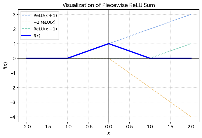
This becomes especially visible in one dimension. Consider

$$f(x) = \text{ReLU}(x+1) - 2\text{ReLU}(x) + \text{ReLU}(x-1)$$

We can examine what happens in different intervals.

If $x < -1$, all three ReLUs are off, so $f(x) = 0$.

If $-1 \le x < 0$, only the first ReLU is active, so $f(x) = x + 1$.

If $0 \le x < 1$, the first two are active, so

$$f(x) = (x+1) - 2x = 1 - x$$

If $x \ge 1$, all three are active, so

$$f(x) = (x+1) - 2x + (x-1) = 0$$

The result is a function that is flat, then rising, then falling, then flat again. A single linear rule cannot do this, because a linear rule has one slope everywhere. This small ReLU construction creates multiple slope regimes because different units switch on and off at different thresholds.

That example is simple, but it captures the mechanism cleanly. ReLU does not need to be smooth to make the model more expressive. It only needs to let different parts of the input space follow different local rules.

From one-dimensional slope changes to multidimensional decision boundaries

In higher dimensions, the same principle becomes geometric.

Each ReLU unit introduces a switching boundary of the form

$$w^\top x + b = 0$$

A layer of many ReLUs creates many such boundaries. Together they partition the input space into regions. Within each region, the network uses one local linear rule. Across regions, it can switch to another. That is how a classifier can bend around structure, isolate pockets of one class, or approximate closed and irregular contours that a single hyperplane could never represent.

This is the moment where the role of nonlinearity becomes concrete. It is not merely that the model becomes more flexible in some vague sense. It is that the model acquires the ability to treat different parts of the space differently.

Why depth matters once nonlinearity is present

A shallow nonlinear network is already much more expressive than a deep linear one, so it is natural to ask why depth helps further. The answer is that once nonlinearity is present, additional layers do not merely add more parameters. They add more stages of transformation.

A shallow ReLU network can already partition the input space into regions and assign different local linear behavior in different regions. That is a major step beyond a linear model. But all of those partitions are still made directly from the original input. Every hidden unit asks its question about the raw input coordinates.

A deeper network changes the situation. The second hidden layer does not operate on the original input directly. It operates on the representation produced by the first hidden layer. But that representation is already a nonlinear function of the input. So from the point of view of the original input space, the second layer is no longer making simple cuts in raw coordinates. It is making cuts in a space that has already been reshaped by previous computation.

This is the key reason depth matters. Each layer can transform the representation, and the next layer can partition that transformed representation again. The network is not just drawing more boundaries. It is repeatedly changing the space in which those boundaries are drawn.

That repeated transformation makes the model far more expressive. Early layers can detect simple patterns. Later layers can combine those patterns into more structured ones. Still later layers can refine those combinations again. In this way, depth gives the network a compositional structure: each stage can build on what earlier stages have already computed, instead of solving the entire problem in one step from the raw input.

This also helps explain why depth can be more efficient than width alone. A shallow network can approximate many complicated functions, but it may need a very large number of units because it must build all of its complexity in one stage. A deeper network can reuse intermediate features across layers, which often allows it to represent structured functions much more compactly.

So once nonlinearity is present, depth matters because it allows the model to repeatedly reshape its representation and then apply new nonlinear partitions to that reshaped space. That is what gives deep networks their layered, compositional power.

A brief note on linear outputs

None of this means every part of a neural network must be nonlinear. In regression, the final output layer is often linear because we want the prediction to remain an unrestricted real number. In classification, the final class scores are often produced by a linear layer and then mapped to probabilities with sigmoid or softmax. The important point is not that every layer must be nonlinear. The important point is that the network must contain nonlinear hidden transformations somewhere in the composition. Without them, the whole system collapses back to one global linear rule.